6 KLRW Category
6.1 Overview
6.2 Computable Add
Let \(\mathcal{C}\) be a preadditive category. Then the computable additive completion of \(\mathcal{C}\), denoted \(\operatorname {CMat}(\mathcal{C})\), has
as objects, lists of elements in \(\mathcal{C}\).
as morphisms, dependent matrices of morphisms in \(\mathcal{C}\). Specifically, if \((A_0, A_1, \ldots , A_n), (B_0, B_1, \ldots , B_m) \in \operatorname {Ob}\big(\operatorname {Mat\_ }(\mathcal{C})\big)\), then
\begin{multline*} \operatorname {Hom}\big((A_0, A_1, \ldots , A_n), (B_0, B_1, \ldots , B_m)\big) \\ = \left\{ \begin{bmatrix} a_{00} & \cdots & a_{0,n-1} \\ \vdots & \ddots & \vdots \\ a_{m-1,0} & \cdots & a_{m-1,n-1} \end{bmatrix} : a_{ij} \in \operatorname {Hom}(A_j, B_i) \right\} \end{multline*}where \(0 \le i \le m-1\) and \(0 \le j \le n-1\).
composition is defined by matrix multiplication
identities are given by the identity matrix
\[ (\mathbb {1}_{(A_0, \ldots , A_m)})_{i, j} = \begin{cases} \mathbb {1}_{A_i} & \text{reinterpreted as an element of }\operatorname {Hom}(A_i, A_j) \text{ by casting along the equality if }i = j \\ 0 & \text{ if }i\ne j \end{cases} \].
There is a fully faithful functor \(G: \mathcal{C}\Rightarrow \operatorname {CMat\_ }(\mathcal{C})\).
There is a fully faithful embedding functor \(F: \operatorname {CMat\_ }(\mathcal{C}) \Rightarrow \operatorname {Mat\_ }(\mathcal{C})\). It is (nonconstructively) essentially surjective, so \(F\) is an equivalence of categories.
Given \(A = (A_0, \ldots , A_n), B=(B_0, \ldots , B_n)\in \operatorname {CMat\_ }(\mathcal{C})\), the computable biproduct of \(A\) and \(B\) is defined by \(A\boxplus _k B = (A_0, \ldots , A_n, B_0, \ldots , B_m)\)
For any \(Z\in \operatorname {CMat\_ }(\mathcal{C})\), the index type, denoted \(\iota _Z\), is the type \(\{ 0, \ldots , (\operatorname {len}(Z)-1)\} \), and the indexing function, \(X_2: \iota _Z\to \mathcal{C}\), is defined by \(X_Z(i) = Z_i\).
Let \(n\in \mathbb {N}\). A positioning of \(1\) black strand with \(n\) red strands is an element of \(\{ 0, \ldots , n+1\} \). Given positionings of \(X\) and \(Y\), the strand set \(StrandSpace_{X, Y} = \mathbb {N}\), representing the number of dots. (Note here that \(\text{StrandSpace}_{X, Y}\) does not depend on \(X\) or \(Y\), but with more black strands it might).
If \(X, Y, Z\) are positionings of \(1\) black strand and \(n\) red strands and \(a\in \text{StrandSpace}_{X, Y}\), \(b\in \text{StrandSpace}_{Y, Z}\), then their composition is given by
Fix a commutative ring \(R\). The \(\operatorname {KLRW}\) category of \(1\) black strand and \(n\) red strands, denoted \(\operatorname {KLRW}\) category of \(1\) black strand and \(n\) red strands, denoted \(\operatorname {KLRW}^R_n\), is given by
\(\operatorname {Ob}(\operatorname {KLRW}^R_n)\) is the set of positionings of \(1\) black strand with \(n\) red strands
\(\operatorname {Hom}(X, Y)\) is the free \(R\)-module generated by \(\text{StrandSpace}_{X, Y}\).
Composition in \(\operatorname {KLRW}^R_n\) is defined by extending the composition of elements of the strand space linearly.
Since each \(\operatorname {Hom}(X, Y)\) is an \(R\)-module and composition is \(R\)-linear, \(\operatorname {KLRW}^R_n\) is \(R\)-linear and thus preadditive.
Let \(\mathcal{C}\) be a preadditive category with a zero object. Then a bounded cochain complex of \(\mathcal{C}\) is a (\(\mathbb {Z}\)-graded) cochain complex \(A^\bullet \) of \(\mathcal{C}\) equipped with a finite set \(S\) called the support, satisfying \(\forall i\in \mathbb {Z}, i\in S \Leftrightarrow A^i\not\cong 0\). Note that \(S\) is uniquely determined by \(A^\bullet \), though included for computability.
6.3 Bounded Cochain Complexes
Let \(\operatorname {BK}^\bullet (\mathcal{C})\) denote the set of bounded cochain complexes in \(\mathcal{C}\). THen there is a function \(F:\operatorname {BK}^\bullet (\mathcal{C})\to K^\bullet (\mathcal{C})\) which forgets the finiteness. Then we equip \(\operatorname {BK}^\bullet (\mathcal{C})\) with the induced category structure of \(F\) which makes \(F\) into a fully faithful functor \(F:\operatorname {BK}^\bullet (\mathcal{C}) \to K^\bullet (\mathcal{C})\).
6.4 Functor data and functor action
6.4.1 Functor data
We will now specify the data needed to define how a braiding functor acts. Let \(R, S, T \in \mathcal{KLRW}\).
The data of a braiding functor is given by the following functions:
In addition to these functions, there must also be proofs that they satisfy \(A_\infty \) relations.
One can understand these functions as specifying how the functor acts on the generating elements of our chain complex category. The action of the functor is as follows.
6.4.2 The action of braiding on generators
Defining \(\beta _0.add\)
Firstly, we may extend the functions acting on \(\mathcal{KLRW}\) to act on \(\operatorname {Add}(\mathcal{KLRW})\) in a linear sense. We define:
by setting:
Defining \(\beta _1.add\)
Extending the remaining two functions requires more care.
For \(\beta _1\), let \(\bigoplus _i A_i\) and \(\bigoplus _j B_j\) be objects in \(\operatorname {Add}(\mathcal{KLRW})\). Let \(f \in \operatorname {Hom}\left(\bigoplus _i A_i, \bigoplus _j B_j\right)\). For each pair \(k, l\), we project \(f\) to its component \(f_{k,l} \in \operatorname {Hom}(A_k, B_l)\). We now create \(g_{k,l} \in \operatorname {Hom}\left(\widehat{\beta }_0\left(\bigoplus _i A_i\right), \widehat{\beta }_0\left(\bigoplus _j B_j\right)\right)\) by extending this morphism. Formally, \(g_{k,l}\) is constructed by composing the canonical projection, the mapped component, and the canonical injection:
Defining \(\beta _2.add\)
For \(\beta _2\), we construct the extension \(\widehat{\beta }_2\) analogously.
6.4.3 The action of braiding on the entire category
Defining \(\beta _0.full\)
Idea
We now define the action of \(\beta \) on a chain complex, i.e. the function
The idea is as follows. The definition takes use of chain complexes of block matrices, i.e. elements in \(K^\bullet AddAddKLRW\). After constructing an element there, we project into \(K^\bullet AddKLRW\).
Let \(A^*\) denote the following cochain complex
For any \(A^i\), consider \(B_i ^*:=\beta _0.add(A^i)\) to be the following cochain complex:
where the left and right bounds are \(l_i\) and \(r_i\).
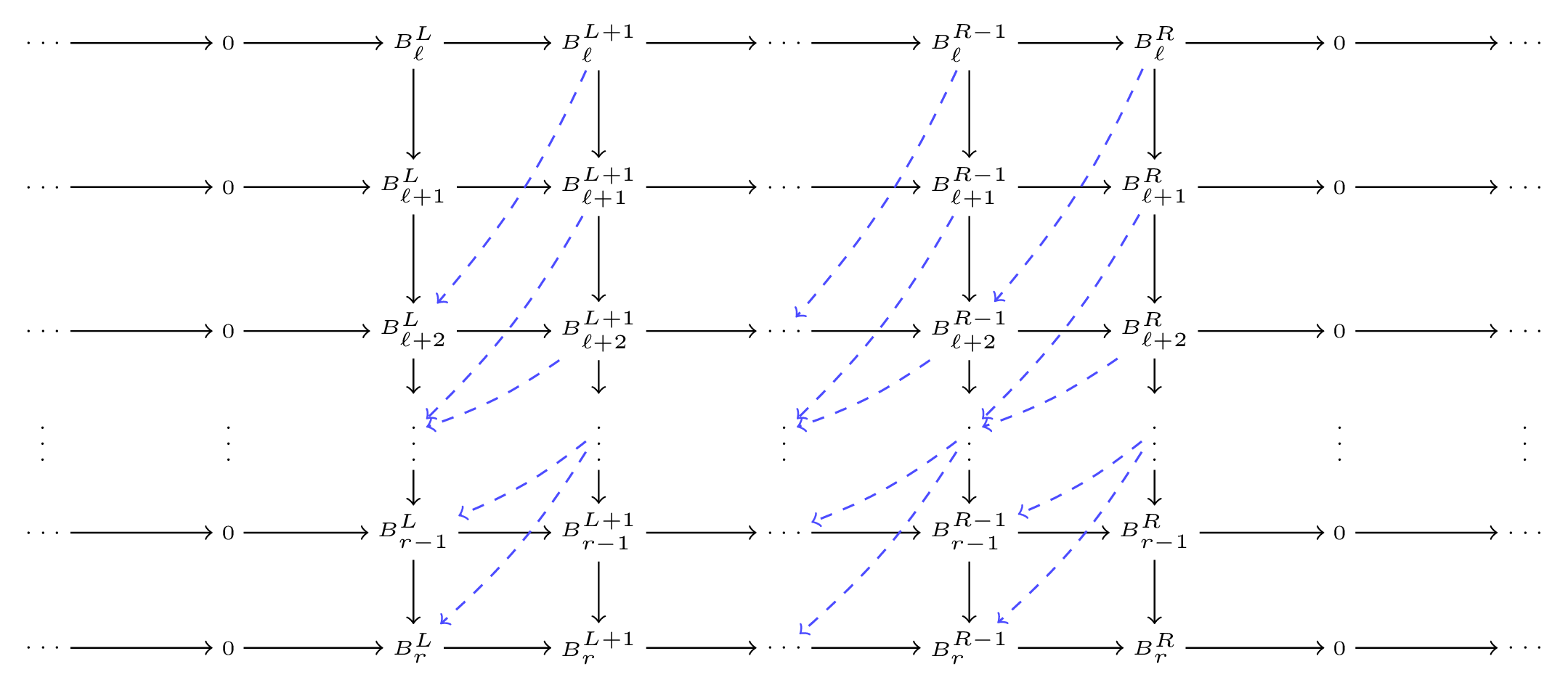
For any \(d^i:A^i -{\gt} A^{i+1}\), we get \(g_i:=\beta _1.add(d^i): B_i ^* \to B_{i+1}^*\). For any two \(d^i:A^i -{\gt} A^{i+1}, d^{i+1}:A^{i+1} -{\gt} A^{i+2}\), we get \(h_i:=\beta _2.add(d^i,d^{i+1}): B_i ^* \to B_{i+2}^*[1]\). This gives rise to the following lattice:
The cochain complex which we want, is then obtained by taking direct sums along the diagonals. The \(A_\infty \)-relations ensure that the resulting object is a cochain complex.
Detailed Construction
Refer to the objects \(A^*, B_i^*, g_i, h_i\) as defined above.
Construct first the following object in \(K^\bullet AddAddKLRW\).
The objects of the chain complex will be \(\mathbb {Z}\)-indexed, where each entry is a list of elements in \(AddKLRW\). For an index \(k\), the element will be the list \(\overline{B}^k:=[B_l ^k, B_{l+1}^{k-1},\dots ,B_r ^{k-r+l}]\).
The bounds are as follows. If \(L_i\) and \(R_i\) is the lower and upper bound of \(B_i\), then our lower bound will be \(min(L_i-i)\) and the upper bound will be \(max(R_i-i)\). The entry will be the \(0\)-list outside the bounds.
The morphisms will be block matrices, where each entry in the matrix is a morphism between entries in the lists (and thus matrices). For \(k\) in these bounds, the morphism \(\overline{B}^k\to \overline{B}^{k+1}\) is given by the lower-triangular matrix of the form
The \(f\)’s are the differentials of \(B^*_i\), the \(g\)’s are the chain maps, and the \(h\)’s are the correction maps. Indices are omitted, but should be possible to infer.
For this to be a differential, it would need to square to 0. This gives rise to the following equations:
These can be interpreted as follows:
Equation 3 ensures \(f\) is a differential.
Equation 4 ensures \(g\) is a chain map: it is \(SF_1\) applied to the input differential \(d^i\).
Equation 5, 6 and 7 are the equations corresponding to \(SF_2\), \(SF_3\) and \(SF_4\) respectively, after simplifying with the source differential relation \(d^{i+1}d^i=0\).
6.4.4 Satisfying A-\(\infty \) axioms
The category \(K^\bullet (\operatorname {Add}(KLRW))\) only has differential \(\mu _1\) and composition \(\mu _2\). Similarly, the braiding functor has no components higher than \(\beta _2\). Therefore the general \([\text{SF}_n]\) axioms for A-\(\infty \) functors reduce to a finite list. They are, in particular, the following axioms.
[SF1]. For all \(f \in \operatorname {Hom}_{\operatorname {KLRW}}(A, B)\),
That is, \(\beta _1(f)\) is a chain map from \(\beta _0(A)\) to \(\beta _0(B)\).
This axiom is automatic from the typing of \(\beta _1\): its codomain consists of morphisms of cochain complexes, which by definition commute with differentials.
[SF2]. For all composable \(f \in \operatorname {Hom}_{\operatorname {KLRW}}(A, B)\) and \(g \in \operatorname {Hom}_{\operatorname {KLRW}}(B, C)\),
[SF3]. For all \(f \in \operatorname {Hom}_{\operatorname {KLRW}}(A, B)\), \(g \in \operatorname {Hom}_{\operatorname {KLRW}}(B, C)\), and \(h \in \operatorname {Hom}_{\operatorname {KLRW}}(C, D)\),
[SF4]. For all (composable) \(f \in \operatorname {Hom}_{\operatorname {KLRW}}(A, B)\), \(g \in \operatorname {Hom}_{\operatorname {KLRW}}(B, C)\), \(h \in \operatorname {Hom}_{\operatorname {KLRW}}(C, D)\), and \(k \in \operatorname {Hom}_{\operatorname {KLRW}}(D, E)\),
Since \(\beta _2\) produces degree \(-1\) maps, their composition has degree \(-2\). This axiom says this composition vanishes. For \(n \geq 5\), all \([\mathrm{SF}_n]\) axioms are identically zero because every term involves either \(\beta _k\) with \(k \geq 3\) or \(\mu _k\) with \(k \geq 3\), both of which are zero.